Hardy-Weinberg Lab
Background
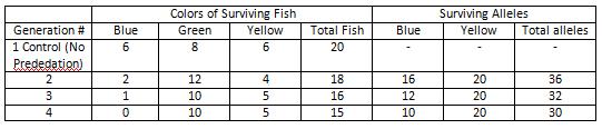
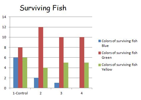
In nature, genes can be mixed creating new gene combinations. To study this process the "straw fish" lab study was performed. The lab was simulating a group of fish in a pond mating with one another sexually sharing their alleles to create various phenotypes. Specifically, the alleles that made up their pigment phenotypes were studied. To simulate random sexual reproduction, all the alleles in a paper bag to be blindly selected in pairs to develop a phenotype for a fish. The alleles were pieces of blue and yellow straws cut up, each color had 20 pieces cut up in the bag. Once selected, the simulated phenotype can be determined by the two alleles B for blue and Y for yellow. The following combinations make up a phenotype: BB= blue, YY= yellow, and BY or YB = green. The Tests were conducted had 4 generations of fish, beginning with the first one being a control and having no predation. To simulate a further, a predation factor was added in. For the Test 1, every other blue fish was eaten. Once all 20 fish were collected and alleles recorded the number of blue fish would be reduced by the predation factor, thus removing their alleles for the surviving alleles count.
Summary #2d
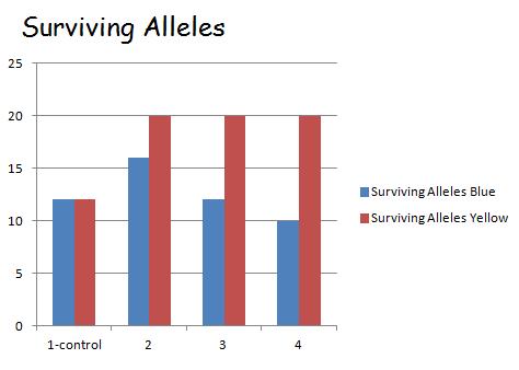
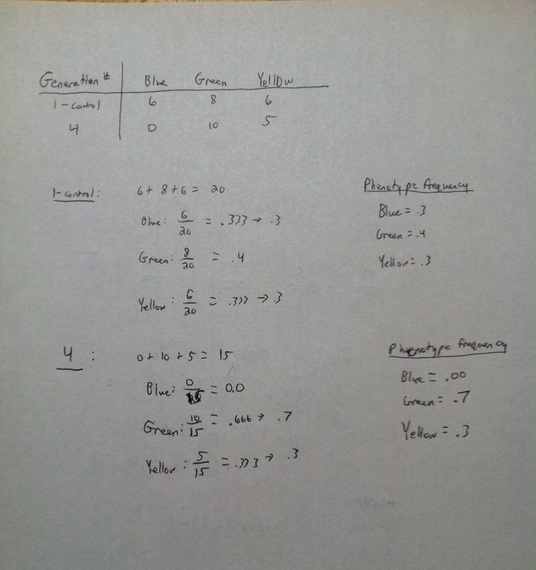
For test 4, the phenotype of the green fish to be able to be camouflaged from predators unlike the blue and yellow which half of which were eaten. This allowed for a consistent rate of blue and yellow fish being eaten by predators to be eaten with their alleles still being carried to the next generation by the green fish. Thus the phenotype and allele frequencies stayed exactly the same as the control had began with. That is having the blue(BB) and yellow (YY) phenotype having a frequency of .25 while the green(BY) having one of .5. The same occurred with the alleles having a B allele frequency of .5 and Y a frequency of .5 .
Hardy-Weinberg Equation
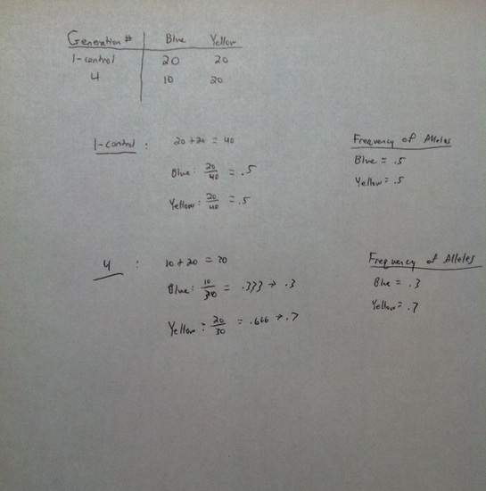
Test 1
In Test 1, there is a variable of having every other blue fish being removed to simulate natural predation of that phenotype color. Once a fish is "eaten" the fish and the alleles that go along with it are removed from that generation and not used in calculations for phenotype and allele counts.
For test 4, the phenotype of the green fish to be able to be camouflaged from predators unlike the blue and yellow which half of which were eaten. This allowed for a consistent rate of blue and yellow fish being eaten by predators to be eaten with their alleles still being carried to the next generation by the green fish. Thus the phenotype and allele frequencies stayed exactly the same as the control had began with. That is having the blue(BB) and yellow (YY) phenotype having a frequency of .25 while the green(BY) having one of .5. The same occurred with the alleles having a B allele frequency of .5 and Y a frequency of .5 .
Hardy-Weinberg Equation
Test 1
In Test 1, there is a variable of having every other blue fish being removed to simulate natural predation of that phenotype color. Once a fish is "eaten" the fish and the alleles that go along with it are removed from that generation and not used in calculations for phenotype and allele counts.
Conditions for Hardy-Weinberg
- no mutation
- random mating
- no selection pressure
- large population size
- no gene flow
Cases 1 and 2
To replicate the random mating and gene distribution through sexual reproduction a small class size gene test was conducted. Each student represented a male or female organism passing down their own alleles to the offspring The student would carry two cards, one dominant and one recessive to begin. Every student would then randomly walk up to another shuffle their two cards and flip the top one over. Their own flipped over card along with the other classmate's cards would be recorded as the first generation. Next, whatever combination the two students created would be used by the student, thus taking on the next generations alleles to be past on again. An example of this is if the two students had two dominant alleles, they would both take on that allele combination by turning in their recessive gene for another dominant one before continuing. After this is repeated for five generations, the frequencies for the different phenotypes can be calculated.
Case 1
Class allele frequencies
p=.6
q=.4
Class genotype frequencies
AA=.36
Aa=.48
aa= .16
Case 2
Class allele frequencies
p=.66
q=.34
Class genotype frequencies
AA=..4356
Aa=..4488
aa= .1156
The case 1 data did not end up matching the initial Hardy-Weinberg due to the adding of the simulated sexual reproduction allowing for randomization. Basically, the randomization allowed for some allele pairs to occur more often causing certain genotype to occur more frequently.
Sources of Error
Some sources of error could drastically change the outcome of this lab. One error of which could be that students did not shuffle their allele cards as well as they should have. Another source could be that the number of alleles total for the class was not the same for case 1 as in case 2 in which the should have been the same, thus a an error could have been caused in the calculations due to an error in data collection.
